Introduction
This repo provides general information about Digital Signal Processing (DSP) alongside a short guide on how to use the LibreDSP library.
Digital Signal Processing (DSP) is the study of techniques and algorithms used to analyze, transform, and synthesize discrete-time signals. A discrete-time signal is simply a sequence of numbers, where each individual number is called a sample. An example of a discrete-time signal is the temperature data captured by a microcontroller from a sensor every \(T\) seconds. Another example of a discrete-time signal is audio sampled and stored as a WAV file.
In DSP, we apply a wide range of algorithm and techniques on discrete-time signals. Generally, these methods can be categorized into two major categories. One is the transform and operations based on the theory of what's called the Fourier Analysis. The second type which is called the statistical DSP, that deals with algorithms developed for random signals. Random signal, in contrast to "deterministic signals", are the ones that are not known in advanced and follow some statistical distributions instead.
The chapters below provide the general theory behind the common DSP algorithms and how they can be applied via the LibreDSP library.
- Chapter 1: Introduction
- Chapter 2: Complex Numbers & Euler's Formula
- Chapter 3: Discrete Fourier Series (DFS) & Discrete Fourier Transform (DFT)
- Chapter 4: Fast Fourier Transform (FFT)
- Chapter 5: Discrete-Time Fourier Transform (DTFT)
- Chapter 6: Z-Transform & Frequency-Selective Digital Filters
- Chapter 7: Digital Filter Design
- Chapter 8: Digital Filter Design: The Windowing Method
- Chapter 9: Statistical Filters
- Chapter 10: Machine Learning for Audio Processing
- Chapter 11: Direction of Arrival (DOA) Estimation
License
This document is licensed under Creative Commons Attribution-ShareAlike 4.0 International. Visit the LICENSE file in the repo for more info.
Complex Numbers & Euler's Formula
Many mathematical operations performed in DSP involve complex number. In this chapter, provides a general overview about these numbers and discusses their connection to what's known as complex exponentials.
A complex number is a number that has the general form \[ a + bj \] where \(a\) and \(b\) are arbitrary real-valued numbers and \(j=\sqrt{-1}\).
An important property of complex numbers is that they form a field. This means that they obey all the familiar rules such as associativity, commutativity, distributivity, and so on, which real numbers also obey. For instance, the following expression is valid for complex numbers: \[ z_1(z_2 + z_3) = z_1z_2 + z_1z_3 \] where \(z_1\), \(z_2\), and \(z_3\) are complex-valued numbers. This is an application of the distributive law.
When dealing with complex numbers, a term that frequently comes up is the complex conjugate. A complex number is a complex conjugate of another complex number if their real parts are the same and their imaginary parts have opposite signs. For instance, numbers \(z_1 = 2 + 3j\) and \(z_2 = 2 - 3j\) are the complex conjugates of each other. Moreover, to show a number is complex conjugate of another number we often use the star symbol. For example, we write \(z_1 = z_2^{\star}\).
What we've seen so far are complex numbers. We also have complex exponentials. These are expressions of the form \(e^{j\theta}\), where \(e\) is Euler's constant, \(j=\sqrt{-1}\), and \(\theta\) is any real-valued number.
Complex exponentials are related to trigonometric functions via Euler's formula. This formula is stated below: \[ e^{j\theta} = \cos(\theta) + j\sin(\theta) \] Where does this formula come from? In one view, Euler's formula can simply be taken as a definition of what it means to raise \(e\) to the power \(j\theta\). In another approach, we first define what it means to raise \(e\) to a general complex number \(z\): \[ e^{z} = \sum_{n=0}^{\infty} \frac{z^n}{n!} = 1 + z + \frac{z^2}{2!} + \frac{z^3}{3!} + \cdots \] Substituting \(z=j\theta\) yields Euler's formula. Either way, we arrive at the same result.
But the question that still remains is: how does this relationship (whether defined or derived) help us?
The answer is that almost all of the familiar rules for real exponentials also hold for complex exponentials. For instance, \[ e^{j(a+b)} = e^{ja}e^{jb}. \]
To prove this, we can rewrite the left-hand side using Euler's formula, apply trigonometric identities, and then use Euler's formula again to obtain the right-hand side.
Differentiation also carries over from real exponentials to complex exponentials. Specifically, \[ \frac{d}{dx}e^{jx}=je^{jx}. \]
Proof:
\[ \frac{d}{dx}e^{jx} = \frac{d}{dx}(\cos x+j\sin x) = -\sin x+j\cos x = je^{jx}. \]
Euler's formula is used extensively in signal processing because it often gives us a shortcut when computing different transforms. More importantly, it allows us to relate certain transforms to other ones, such as the Discrete-time Fourier Transform (DTFT) to the Z-transform, or the Continuous-time Fourier Transform (CTFT) to the Laplace transform.
Discrete Fourier Series (DFS) & Discrete Fourier Transform (DFT)
In this chapter we will discuss Discrete Fourier Series (DFS) and its usage which is to decompose a discrete-time signals in terms of complex exponentials. Afterwards, we will see a closely related operation called the Discrete Fourier Transform (DFT). As we will see, the computations performed for DFS is, in fact, identical to DFT and their difference is merely the interpretation of the results.
Consider a periodic discrete-time signal \(x[n]\) with period \(N_0\). That means
\[ x[n+N_0]=x[n]. \]
Where \(N_0\) is an integer. We can rewrite such signals as sums of complex exponentials: \[ \boxed{x[n]=\sum_{k=0}^{N_0-1}a_ke^{jk\omega_0n}, \qquad \omega_0=\frac{2\pi}{N_0}}. \]
This is called the Discrete Fourier Series (DFS) expansion of the signal \(x[n]\). Expanding the sum gives us \(N_0\) equations with \(N_0\) unknowns. In matrix notation, we have \(Ax=b\), where \(A\) is a matrix consisting of complex exponential terms, \(x\) is a vector containing the unknown coefficients that we are trying to find, and \(b\) contains the values of the signal at different samples. In other words, DFS is merely a system of \(N\) equation and \(N\) unknowns.
Can we apply standard Gaussian elimination to solve such systems?
The answer is yes. Complex numbers form a field, and Gaussian elimination works on any matrix whose entries belong to a field. Hence, it can be used to solve \(Ax=b\).
Even though Gaussian elimination gives us a method for computing the DFS coefficients, in practice we exploit a special property of the matrix \(A\) and compute the coefficients using the closed-form formula: \[ a_k=\frac{1}{N_0}\sum_{n=0}^{N_0-1}x[n]e^{-jk\omega_0n}, \qquad \omega_0=\frac{2\pi}{N_0}. \]
As an example, suppose we want to compute the DFS coefficients of the periodic signal \(x[0]=2\), \(x[1]=1\), \(x[2]=3\), and \(x[3]=3\) (with \(x[n]=x[n \bmod 4]\)).
\[ k=0 \rightarrow e^{j2\pi(n)(0)/4} = 1,1,1,1 \rightarrow a_0=\frac{1}{4}(2+1+3+3)=\frac{9}{4} \]
\[ k=1 \rightarrow e^{j2\pi(n)(1)/4} = 1,-j,-1,j \rightarrow a_1=\frac{1}{4}(2-j-3+3j) = -\frac{1}{4}+j\frac{1}{2} \]
\[ k=2 \rightarrow e^{j2\pi(n)(2)/4} = 1,-1,1,-1 \rightarrow a_2=\frac{1}{4}(2-1+3-3) = \frac{1}{4} \]
\[ k=3 \rightarrow e^{j2\pi(n)(3)/4} = 1,j,-1,-j \rightarrow a_3=\frac{1}{4}(2+j-3-3j) = -\frac{1}{4}-j\frac{1}{2} \]
An interesting observation is that, after expanding the signal in terms of complex exponentials, we obtain
\[ x[n] = \frac{9}{4}e^{j2\pi(0)n/4} + \left(-\frac{1}{4}+j\frac{1}{2}\right)e^{j2\pi n/4} + \frac{1}{4}e^{j4\pi n/4} + \left(-\frac{1}{4}-j\frac{1}{2}\right)e^{j6\pi n/4} \]
\[ = \frac{9}{4}e^{j2\pi(0)n/4} + \left(-\frac{1}{4}+j\frac{1}{2}\right)e^{j2\pi n/4} + \left(-\frac{1}{4}-j\frac{1}{2}\right)e^{-j2\pi n/4} + \frac{1}{4}e^{j\pi n} \]
\[ = \frac{9}{4} - \frac{1}{2}\cos\left(\frac{\pi n}{2}\right) - \sin\left(\frac{\pi n}{2}\right) + \frac{1}{4}\cos(\pi n) \]
By rearranging the terms, we expressed the signal as a sum of harmonically related real-valued sines and cosines.
Note 1: In general, for any real-valued signal, the DFS coefficients satisfy \[ \boxed{a_{N-k}=a_k^{\ast}}, \] where \(N\) is the period and the operator \(^{\ast}\) denotes complex conjugation. As a consequence, we can pair the \(k\) and \(N-k\) terms together to obtain real-valued sinusoids.
Note 2: The DFS we discussed assumes that we have a periodic function, and the coefficients of DFS allow us to decompose that periodic function as a sum of complex exponentials. An identical operation to DFS is called the Discrete Fourier Transform (DFT). DFT has exactly the same formulas as DFS, but there, we assume that we are decomposing a finite-length signal by complex exponentials. Otherwise, all the mathematics is the same. In other words, we can treat the finite-length signal as one period of a periodic function, and in that case DFS and DFT become identical.
In the next chapter, we will discuss an algorithm called the Fast Fourier Transform (FFT) which efficiently computes the DFS or DFT coefficients, as well as reconstructs signals using those coefficients.
Fast Fourier Transform (FFT)
In the previous chapter we saw that the DFS allowed us to decompose a periodic discrete-time signal and write it as a sum of complex exponentials. As we also discussed, the computations performed for the DFS are identical to what's performed for the discrete Fourier transform (DFT). For the DFS, we implicitly assume that the signal we apply the DFS on is periodic. For the DFT in contrast, we assume that we have a finite sequence of numbers. However, the computations for the two transforms are the same, and the difference is merely a conceptual one. In this chapter, we develop our discussion for the DFT, but everything works the same for the DFS as well.
To recap, via the DFT, a signal can be written via the following expression. \[ x[n]=\sum_{k=0}^{N_0-1}a_ke^{jk2\pi n / N_0} \] Where the coefficients \(a_k\)'s are computed via: \[ a_k=\frac{1}{N_0}\sum_{n=0}^{N_0-1}x[n]e^{-jk2 \pi n / N_0} \] Notice that here we have \(N_0\) such coefficients, and each one requires a sum from \(0\) to \(N_0-1\) to compute. Therefore, if we perform these operations via a computer program, we say that its time complexity is \(O(N_0^2)\). The symbol \(O\) is called Big O notation, and it tells us how the complexity of the algorithm grows as a function of the input size. For computing the coefficients of the DFS, we see that if we have \(N_0\) samples, then computing all \(N_0\) coefficients, each requiring a sum of \(N_0\) terms, takes \(N_0 \times N_0 = N_0^2\) steps. Therefore, we say the time complexity is \(O(N_0^2)\). A time complexity of \(O(N^2)\) is generally not desirable for algorithms, and we often look for algorithms that work in linear or logarithmic complexity instead. As it turns out, an algorithm called the Fast Fourier Transform can compute the \(a_k\) coefficients (and also reconstruct the signal \(x[n]\) from those coefficients) in \(O(N_0 \log N_0)\) time complexity. This is a great improvement over a naive computation of the DFT coefficients and is used extensively in any application that requires the DFT. In what follows, we will explore a classic variant of the FFT called radix-2.
Radix-2 FFT Algorithm
The radix-2 FFT algorithm computes the DFT of a sequence whose size is a power of 2. Therefore, if the signal is not a power of two, we can make it such a sequence by appending zeros to the end of the sequence until its size is the next power of 2. We now assume that the sequence \(x[n]\) has a size that is a power of 2. Its DFT coefficients are, again, computed as:
\[ a_k=\frac{1}{N_0}\sum_{n=0}^{N_0-1}x[n]e^{-j2\pi kn/N_0}, \qquad k=0,1,\ldots,N_0-1. \]
We can rewrite the above expression and separate the sum into two parts: one part, a sum over even-indexed samples, and another over odd-indexed samples. \[ a_k= \frac{1}{N_0}\sum_{m=0}^{N_0/2-1}x[2m]e^{-j2\pi k(2m)/N_0}+ \frac{1}{N_0}\sum_{m=0}^{N_0/2-1}x[2m+1]e^{-j2\pi k(2m+1)/N_0} \]
Notice for the even term, we can write the exponential term as: \[ e^{-j2\pi k(2m)/N_0} =e^{-j2\pi km/(N_0/2)} \]
For the odd term we can write: \[ e^{-j2\pi k(2m+1)/N_0}= e^{-j2\pi k/N_0}e^{-j2\pi km/(N_0/2)} \]
Using these two substitutions, we can then write the sum as: \[ a_k=\frac{1}{N_0}\sum_{m=0}^{N_0/2-1}x[2m]e^{-j2\pi km/(N_0/2)}+ e^{-j2\pi k/N_0} \frac{1}{N_0}\sum_{m=0}^{N_0/2-1}x[2m+1]e^{-j2\pi km/(N_0/2)} \]
If we call the first sum \(E_k\) and the latter one \(O_k\), then we have: \[ a_k=E_k+e^{-j2\pi k/N_0}O_k \]
The term \(e^{-j2\pi k/N_0}\) is called the twiddle factor. Notice that \(E_k\) is closely related to the DFT of the even samples, and \(O_k\) is related to the DFT of the odd samples. Specifically, the DFT of the even samples is: \[ D_e[k]= \frac{2}{N_0} \sum_{m=0}^{N_0/2-1} x[2m]e^{-j2\pi km/(N_0/2)}, \qquad k=0,1,\ldots,N_0/2-1. \]
Comparing this to \(E_k\), we have: \[ E_k=\frac{1}{2}D_e[k\bmod(N_0/2)] \]
The same applies for \(O_k\) and the DFT of the odd samples. If we denote the DFT of the odd samples as \(D_o\), then we have: \[ O_k=\frac{1}{2}D_o[k\bmod(N_0/2)] \]
This means that \(E_k\) is the DFT of the even-indexed samples, scaled by a factor of \(1/2\), up to \(k=N_0/2-1\). Since the DFT of a sequence of length \(N_0/2\) is periodic with period \(N_0/2\), for \(k\) from \(N_0/2\) up to \(N_0-1\), the DFT coefficients repeat. The same applies to \(O_k\) and the DFT of the odd-indexed samples.
Therefore: \[ E_{k+N_0/2}=E_k \] \[ O_{k+N_0/2}=O_k \]
For the second half of the DFT coefficients, we replace \(k\) by \(k+N_0/2\) in \(a_k=E_k+e^{-j2\pi k/N_0}O_k\). Using the above relations and \[ e^{-j2\pi(k+N_0/2)/N_0} =-e^{-j2\pi k/N_0} \] we obtain:
\[ \boxed{ \begin{aligned} a_k &= E_k+e^{-j2\pi k/N_0}O_k \\ a_{k+N_0/2} &= E_k-e^{-j2\pi k/N_0}O_k \end{aligned} } \qquad k=0,1,\ldots,N_0/2-1. \]
This is a recursive definition, and it tells us that the DFT of a sequence of size \(N_0\) can be computed via the DFT of two sequences, each with size \(N_0/2\).
To see this concretely, assume we have a function called \(fft(...)\) that computes the FFT of the sequence that is passed to it as its argument. The tree execution of this function would be:
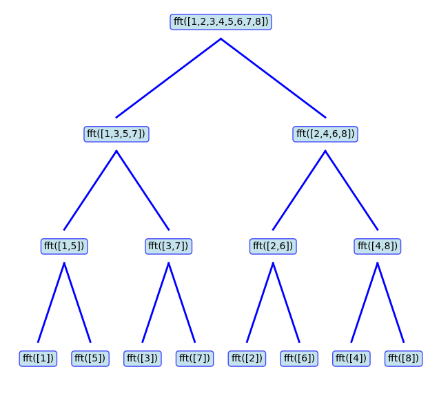
As the figure shows, to compute the FFT of the sequence \([1,2,\ldots,8]\), the program merges the results obtained by calling the FFT function on the sequences \([1,3,5,7]\) and \([2,4,6,8]\). Also, to compute the FFT of each one, the program has to branch out further and compute the FFT of its odd- and even-indexed elements. This recursive call continues until the program hits the base case, which is the task of computing the FFT of a single element. This FFT is trivial to compute, and it's just the value itself. To see that, \(N_0=1\), the only term is \(n=0,k=0\): \[ a_0=x[0]e^{-j2\pi (0)(0) / 1} = x[0] \]
Note: It is a convention to compute the DFT coefficients in radix-2 implementations as: \[ a_k=\sum_{n=0}^{N_0-1}x[n]e^{-jk2 \pi n / N_0} \] In this form, the formula does not have the scaling factor \(\frac{1}{N_0}\) before the sum (in contrast to the formula we had for the DFT). However, for the reconstruction of the signal, that is executing the inverse DFT, we use: \[ x[n]=\frac{1}{N_0} \sum_{k=0}^{N_0-1}a_ke^{jk2\pi n / N_0} \]
The following code creates a discrete-time signal and applies the FFT on it via LibreDSP:
use libredsp::signal::Signal;

fn main() {
    let signal = Signal::new(vec![1.0, 0.0, 0.0, 0.0]);
    // Apply FFT
    let spectrum = signal.fft();
    println!("Result of the FFT: {:?}", spectrum);
}
The output of the code is as follows:
Result of the FFT: [Complex { re: 1.0, im: 0.0 }, Complex { re: 1.0, im: 0.0 }, Complex { re: 1.0, im: 0.0 }, Complex { re: 1.0, im: 0.0 }]
Discrete-Time Fourier Transform (DTFT)
The DFS and DFT we discussed in Chapter 3 were great tools for decomposing arbitrary discrete-time signals in terms of complex exponentials. We then saw an efficient way to compute those transforms via the FFT in Chapter 4. A major limitations of the DFT and DFS though, is that the coefficients we obtain by computing those transform depend heavily on the length of signals. In other words, the DFT and DFS operations of two signals are only comparable (and can be added and subtracted, etc) if the underlying discrete-time signals have the same length. To overcome this limitation, we can zero-pad two arbitrary signals to have the same length, and then compute the DFT or DFS (via the FFT) for them. For the analytical purposes though, it is often suitable to add infinite zeros, in the limit sense, and then compute the DFT or DFS. By doing so, we obtain what's called the Discrete-time Fourier Transform (DTFT) of the signal. In this chapter we briefly introduce this transform and then we will see how we can obtain it in LibreDSP via the FFT operation.
Let us start with an aperiodic discrete-time signal. To obtain the DTFT of the signal, the basic idea is to construct a periodic signal by appending zeros to an aperiodic signal and then repeating that signal to make it periodic. We then apply DFS on this periodic signal. In this setup, as the number of appended zeros approaches infinity, the DFS becomes the DTFT.
Let \(x[n]\) be an aperiodic signal that is nonzero only for \[ N_1 \le n \le N_2. \]
Choose a period \(N \ge N_2-N_1+1\) and construct the periodic extension of \(x[n]\) by repeating one period that contains the entire nonzero portion of the signal. The DFS coefficients are
\[ a_k = \frac{1}{N}\sum_{n=0}^{N-1}x[n]e^{-jk\omega_0n} = \frac{1}{N}\sum_{n=-\infty}^{\infty}x[n]e^{-jk\omega_0n} = \frac{1}{N}X(e^{j\omega_0k}), \]
where \[ \omega_0=\frac{2\pi}{N}, \] and \(X(e^{j\omega})\) is a function of \(\omega\) that we would call the 'DTFT'.
The synthesis equation then becomes
\[ x[n] = \sum_{k=0}^{N-1}a_ke^{jk\omega_0n} = \frac{1}{N}\sum_{k=0}^{N-1}X(e^{j\omega_0k})e^{jk\omega_0n}. \]
Using the relation \[ \omega_0=\frac{2\pi}{N}, \] we obtain
\[ x[n] = \frac{1}{2\pi} \sum_{k=0}^{N-1} X(e^{j\omega_0k}) e^{jk\omega_0n} \omega_0. \]
As \(N\rightarrow\infty\), we have \(\omega_0\rightarrow0\), and the sum becomes an integral:
\[ x[n] = \frac{1}{2\pi} \int_0^{2\pi} X(e^{j\omega}) e^{j\omega n} d\omega. \]
In summary, an aperiodic discrete-time signal can be expressed as an integral of complex exponentials through the Discrete-Time Fourier Transform (DTFT):
Synthesis \[ \boxed{x[n] = \frac{1}{2\pi} \int_0^{2\pi} X(e^{j\omega}) e^{j\omega n} d\omega}. \]
Analysis \[ \boxed{X(e^{j\omega}) = \sum_{n=-\infty}^{\infty} x[n] e^{-j\omega n}}. \]
The analysis equation computes the DTFT \(X(e^{j\omega})\) from the signal \(x[n]\), while the synthesis equation reconstructs \(x[n]\) from its DTFT.
Note 1: In the derivation the DTFT, this step:
\[ x[n] = \frac{1}{2\pi} \int_0^{2\pi} X(e^{j\omega}) e^{j\omega n} d\omega \]
is only valid if we can expand it as:
\[ x[n] = \frac{1}{2\pi} \int_0^{2\pi} \sum_{m=-\infty}^{\infty} x[m] e^{-j\omega m} e^{j\omega n} d\omega = \sum_{m=-\infty}^{\infty} x[m] \left( \frac{1}{2\pi} \int_0^{2\pi} e^{j\omega (n-m)} d\omega \right) \] The inner integral evaluates to \(1\) when \(m = n\) and to \(0\) otherwise. This leaves only the \(m = n\) term in the sum, resulting in \(x[n]\).
As we can see, the equation above requires interchanging the sum and integral. For discrete-time signals with finite length this is valid, but it is not for an arbitrary infinite-length signal. However, if a signal is absolutely summable, meaning that the sum of its absolute values is finite:
\[ \sum_{n=-\infty}^{\infty} |x[n]| < \infty \]
then we can safely interchange the sum and integral (for both finite and infinite length signals). Therefore, absolute summability is a sufficient condition for the DTFT to exist.
Note 2: The conjugate property for real-valued signals that we saw for the DFS also holds for the DTFT. That is, \[ \boxed{X(e^{j\omega}) = X^*(e^{-j\omega})}. \]
For discrete-time complex exponentials (as well as discrete-time sinusoids), adding \(2\pi\) to the frequency gives the same function, i.e., \[ e^{j(\omega+2\pi)n}=e^{j\omega n}. \] As a result, the DTFT \(X(e^{j\omega})\) is always periodic with period \(2\pi\). Hence, to plot the result of DTFT, it is enough plot only \(2\pi\) interval of the graph.
Note 3: A useful identify used when computing many DTFTs is the geometric series: \[ 1+a+a^2+\cdots=\frac{1}{1-a}, \qquad |a|<1. \]
The above relation is valid for both real-valued as well as complex-valued numbers.
An example of DTFT
Find the DTFT of the signal \[ x[n]= \begin{cases} a^n, & n\ge0,\\ 0, & n<0, \end{cases} \] where \( |a|<1 \).
Answer: We use the DTFT analysis equation: \[ \begin{aligned} X(e^{j\omega}) &= \sum_{n=-\infty}^{\infty}x[n]e^{-j\omega n} = \sum_{n=0}^{\infty}a^ne^{-j\omega n} \\ &= \sum_{n=0}^{\infty}(ae^{-j\omega})^n = \frac{1}{1-ae^{-j\omega}}. \end{aligned} \]
Convolution Theorem
Given two signals \(x[n]\) and \(y[n]\) with DTFTs \(X(e^{j\omega})\) and \(Y(e^{j\omega})\), if we multiply their DTFTs, i.e., compute \(X(e^{j\omega})Y(e^{j\omega})\), what operation in the time domain does this correspond to? Said differently, what's the inverse DTFT of \(X(e^{j\omega})Y(e^{j\omega})\)? The answer is the convolution (you can find nice visualizations of the convolution operation online). More specifically, the convolution theorem states that
\[ \boxed{r[n] = x[n]*y[n] = \sum_{k=-\infty}^{\infty}x[k]y[n-k]}. \]
Then \[ \boxed{\mathcal{F}\{x[n]*y[n]\} = X(e^{j\omega})Y(e^{j\omega})}. \]
Where \(*\) is the convolution operator.
In short, the convolution theorem tells us that multiplication in the frequency domain corresponds to convolution in the time domain.
Conversely, multiplication in the time domain corresponds to convolution in the frequency domain (more precisely, "periodic convolution" which is the convolution over an interval of length \(2\pi\)), scaled by \(1/(2\pi)\):
\[ \mathcal{F}\{x[n]y[n]\} = \frac{1}{2\pi} \int_0^{2\pi} X(e^{j\theta}) Y(e^{j(\omega-\theta)}) d\theta. \]
Multiplying two signals in the frequency domain can be thought of as modifying the frequency content of a signal. For example, whenever we multiply the DTFT of a signal by the DTFT of a rectangle function, the result is a function whose frequency content is preserved up to a cutoff frequency, while higher frequencies are removed. This operation is referred to as low-pass filtering. Also, multiplication by the rectangle function in the frequency domain performs ideal low-pass filtering. It passes all frequencies up to a certain cutoff frequency, and completely blocks higher ones.
Other common filters include high-pass, band-pass, band-stop, and all-pass (which only add phase shifts) filters.
To summarize, the result of multiplying two signals in the frequency domain can be obtained in two equivalent ways:
- Compute the DTFT of the signal, multiply it by the DTFT of a second function, and then compute the inverse DTFT.
- Convolve the signal with \[ g[n]=\mathcal{F}^{-1}\{G(e^{j\omega})\}, \] where \(G(e^{j\omega})\) is the DTFT of the second function.
Note: In the coming chapters, we only use the convolution theorem we just saw, which holds for the DTFT. However, for the sake of completeness, a small note about convolution operation. The DFS (or DFT) we discussed in the previous subsection also has a convolution theorem associated with it. There, however, the convolution is of a different form called a circular convolution. Circular convolution of two sequences \(x[n]\) and \(y[n]\), both of length \(N\), is defined as follows (note that circular convolution is defined for two sequences of the same length): \[ x[n] \circledast y[n] = \sum_{m=0}^{N-1} x[m] y[(n - m) \bmod N] \] As the expression above suggests, whenever the index \((n-m)\) is negative or greater than or equal to \(N\), the \(\bmod\) operator brings it back into the range \(0\) to \(N-1\). In other words, the convolution "wraps around" for values smaller than \(0\) and larger than or equal to \(N\). Hence, the sum from \(m=0\) to \(N-1\) always multiplies some values of both sequences for a given value of \(n\). Unlike normal convolution, there is no case where the two sequences fail to overlap and some parts of the signals get multiplied by zero. To turn the circular convolution into a normal (linear) convolution, we can artificially add zeroes ("zero-padding") to both sequences so that each has length at least \(N_1 + N_2 - 1\), where \(N_1\) and \(N_2\) are the original lengths of the two sequences. Afterwards, the circular convolution computed on these zero-padded sequences equals the linear convolution, just like the convolution we have for the DTFT, for all values of \(n\) in \([0, N_1 + N_2 - 1)\).
The Delta Function
We now re-introduce an the Delta or the Impulse function, and discuss its properties in light of the new concepts we have convered. To recap, mathematically this function is defined as:
\[ \boxed{\delta[n]= \begin{cases} 1, & n=0,\\ 0, & n\neq0. \end{cases}} \]
Its DTFT is
\[ \mathcal{F}\{\delta[n]\} = \sum_{n=-\infty}^{\infty} \delta[n]e^{-j\omega n} = 1. \]
The discrete-time delta also satisfies the convolution identity
\[ \delta[n]*x[n]=x[n]. \]
Frequency Selective Systems
The convolution theorem told us what happens if we convolve two signals in the time domain, i.e., the effect of convolution is same as multiplication of two signal's DTFTs \(A(\omega)B(\omega)\) and then taking inverse DTFT of the result \(\mathcal{F}^{-1} \{ A(\omega)B(\omega) \} \).
We are now ready to talk about systems that receive an input signal \(x[n]\) and produce an output signal \(y[n]\), such that \(y[n] = x[n] * h[n]\), where \(h[n]\) is a function intrinsic to the system. By the convolution theorem, the spectrum of \(y[n]\), denoted by \(Y(e^{j\omega})\), is given by \(Y(e^{j\omega})=H(e^{j\omega})X(e^{j\omega})\), where \(H(e^{j\omega})\) is the DTFT of \(h[n]\). The function \(H(e^{j\omega})\) is also called the transfer function of the system. Such systems perform frequency-selective filtering on the input signal.
Something interesting happens if we choose the input to such a system to be the delta function.
Consider \(x[n]=\delta[n]\). Then \(y[n]\) is computed as follows:
\[ y[n] = \delta[n] * h[n] = h[n] \]
That is why signal \(h[n]\) is called the impulse response and can completely characterize the system. Because, once we have \(h[n]\), we can compute the output of the system for any arbitrary input \(x[n]\) as: \[ y[n] = x[n]*h[n]. \]
Same analysis in the frequency domain is as follows: If input \(x[n] = \delta[n]\), its spectrum is \(X(e^{j\omega})=1\), so
\[ Y(e^{j\omega})=H(e^{j\omega}). \]
Taking the inverse DTFT gives
\[ y[n] = \mathcal{F}^{-1}\{H(e^{j\omega})\} = h[n]. \]
Which is exactly the same function, \(h[n]\), the impulse response.
Example: As an important example of such a system, consider a system that performs ideal low-pass filter. The frequency response of such a filter is:
\[ H(e^{j\omega}) = \begin{cases} 1, & |\omega| < \omega_c \\ 0, & \omega_c < |\omega| \leq \pi \end{cases} \]
where \(\omega_c\) is the cutoff frequency, between \(0\) and \(\pi\).
The inverse DTFT of this expression yields:
\[ h[n] = \frac{1}{2\pi} \int_{-\pi}^{\pi} H(e^{j\omega})e^{j\omega n}d\omega = \frac{1}{2\pi} \int_{-\omega_c}^{\omega_c} e^{j\omega n}d\omega = \frac{\sin(\omega_c n)}{\pi n} \]
For \(n \neq 0\),
\[ h[n] = \frac{\sin(\omega_c n)}{\pi n}. \]
At \(n=0\), we have \(h[0] = \omega_c / \pi\), since the value \(\omega_c / \pi\) can be obtained by expressing the function as a continuous function and applying L'Hôpital's rule.
Using the definition of the normalized sinc function,
\[ \operatorname{sinc}(x)=\frac{\sin(\pi x)}{\pi x}, \]
this can be written as
\[ \boxed{ h[n] = \frac{\omega_c}{\pi} \operatorname{sinc}\left(\frac{\omega_c n}{\pi}\right) } \]
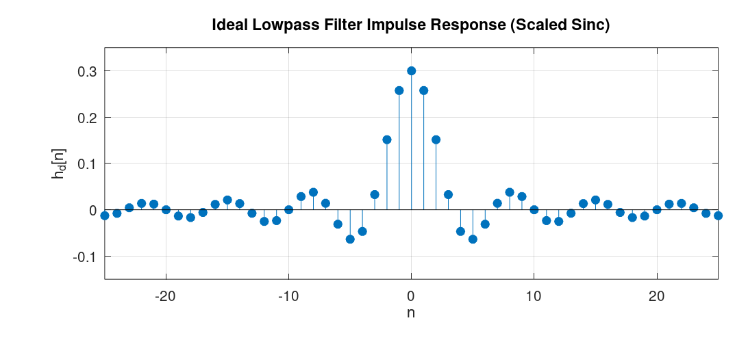
The graph of this function is depicted below:
Additional properties
Two additional properties of the DTFT are linearity and time shifting.
Linearity \[ \boxed{ax[n]+by[n] \longrightarrow aX(e^{j\omega})+bY(e^{j\omega})}. \]
Time shifting \[ \boxed{x[n-n_0] \longrightarrow e^{-j\omega n_0}X(e^{j\omega})}. \]
For example, let \[ x[n]\longrightarrow X(e^{j\omega}), \qquad y[n]\longrightarrow Y(e^{j\omega}). \]
If \[ z[n]=2x[n]+3y[n], \] then by linearity, \[ Z(e^{j\omega}) = 2X(e^{j\omega}) + 3Y(e^{j\omega}). \]
Lastly, a useful theorem in DSP:
Uncertainty principle: A bandlimited signal, whose frequency content is zero above and below certain frequencies, cannot be time-limited, that is, its content in the time domain cannot be zero outside a finite range of indices [1].
As an example, consider the ideal-low pass filter we mentioned in the previous subsection. As we saw, the frequency response of such a filter is limited to the range \([-\omega_c,\omega_c]\), but the impulse response extends over all indices from \(-\infty\) to \(+\infty\). Therefore it is not both time-limited and bandlimited. Conversely, it can also be shown that a rectangle function in the time domain has a DTFT that is sinc-like, extending over all frequencies. This confirms the same conclusion from the other direction, that is, a time-limited signal cannot be bandlimited either. The uncertainty principle can also be useful for memorizing DTFT pairs. For instance, when a signal is time-limited, we can be sure that its DTFT is nonzero throughout the entire frequency range \([-\pi,\pi]\).
The definition of the DTFT, we have seen, is defined in a limit sense. We can, however, estimate its graph by zero-pad a signal with a large number of zeroes and then apply FFT. In LibreDSP, it can be done via:
use libredsp::signal::Signal;

fn main() {
    let mut signal = Signal::new(vec![1.0, 0.0, 0.0, 0.0]);
    println!("Signal: {:?}", signal.clone().to_vec());

    // Apply FFT
    signal.zero_pad(1000);
    let dtft = signal.fft();
    println!("The DTFT {:?}", dtft);
}
References
[1]: Chapter 7 - Vetterli M, Goyal VK, Kovačević J. Foundations of signal processing. Cambridge University Press; 2014 Sep.
Z-Transform
In this chapter, we will introduce the bilateral Z-transform, which is often referred to as simply the Z-transform. As we will see, the DTFT we talked about in the previous chapter is a special case of the bilateral Z-transform. Afterwards, we will discuss a variant of it called the unilateral Z-transform, which allows us to solve linear constant-coefficient difference equations. Lastly, we will discuss the relationship between the solution obtained via the unilateral Z-transform and the DTFT as well.
Bilateral Z-transform
The bilateral Z-transform of a discrete-time signal \(x[n]\) is defined as \[ \boxed{X(z) = \sum_{n=-\infty}^{\infty} x[n]z^{-n}} \] where \(z\) is a complex variable.
If we let \[ z=re^{j\omega}, \]
then
\[ X(re^{j\omega}) = \sum_{n=-\infty}^{\infty} x[n] (r e^{j\omega} )^{-n} = \sum_{n=-\infty}^{\infty} (x[n]r^{-n})e^{-j\omega n} \]
which means that the bilateral Z-transform is simply the DTFT of the signal \(x[n]r^{-n}\). For \(r=1\), we get the actual DTFT.
The presence of \(r\) gives us an extra degree of freedom. As a consequence, the bilateral Z-transform exists for signals such as exponentially growing signals, that normally do not have a DTFT. For these signals, the extra degree of freedom (via an exponential) results in the signal to become well-behaved and causes the summation to have a finite value.
Some Properties
The set of values of \(z\) for which the bilateral Z-transform converges is called the Region of Convergence (ROC).
As an example, consider \[ x[n]=a^nu[n]. \]
Its bilateral Z-transform is \[ X(z) = \sum_{n=-\infty}^{\infty} a^nu[n]z^{-n} = \sum_{n=0}^{\infty} (az^{-1})^n. \]
The geometric series converges if \[ |az^{-1}|<1, \] or equivalently, \[ |z|>|a|. \]
Therefore, \[ X(z) = \frac{1}{1-az^{-1}} = \frac{z}{z-a}, \qquad |z|>|a|. \]
The ROC of the bilateral Z-transform is illustrated on the z-plane as depicted below (to have a concrete example the figure assumes \(a = 0.8 \)):
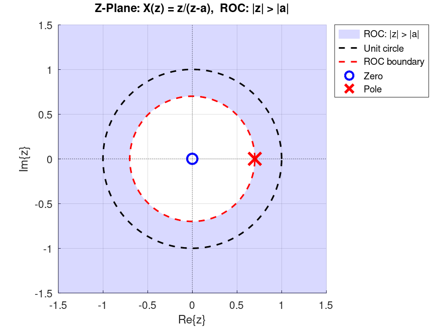
As the figure shows, the shaded area, which is \(|z| > 0.8\), is the ROC of \(X(z)\) we computed earlier. In the figure, you can also notice the location of the pole and the zero. A zero is a root of the numerator of \(X(z)\), and a pole is a root of the denominator of X(z), after simplifying X(z) and cancelling any common roots between the numerator and denominator.
Note: A different sequence can result in the same bilateral Z-transform expression but have a different ROC. Consequently, when we refer to the Z-transform of a function, we should always specify its corresponding ROC as well.
Many other properties of the DTFT (such as linearity and convolution) carry over to the bilateral Z-transform as well. Specifically, linearity holds just like it does for the DTFT. The convolution of two signals also corresponds to the multiplication of their Z-transforms, with one small caveat: the ROC of the resulting Z-transform is the intersection of the ROCs of the Z-transforms of each signal.
Unilateral Z-Transform
A related but different type of transform from the bilateral Z-transform, is called the unilateral Z-transform. One of the primary usages of the unilateral Z-transform is to solve linear constant-coefficient difference equations (LCCDEs). The expression for the unilateral Z-transform is as follows: \[ \boxed{X(z) = \sum_{n=0}^{\infty} x[n]z^{-n}}. \]
When applied to the signal \(x[n]\), the unilateral Z-transform can be thought of as the bilateral Z-transform of the signal \(x[n]\) multiplied by the unit step function, that is, the bilateral Z-tranform of \(x[n]u[n]\). Furthermore, for a rational Z-transform, the ROC is the region outside the outermost pole. Most properties are identical for the bilateral and unilateral Z-transforms, such as linearity. The convolution property also holds provided both signals are zero for \(n<0\).
For the unilateral Z-transform, the time-shifting property is \[ \boxed{x[n-1] \Longleftrightarrow zX(z)-zx[-1]}. \]
This property allows us to solve LCCDEs with initial conditions.
Solving LCCDEs via Unilateral Z-transform
One of the primary applications of the unilateral Z-transform is to find solutions to LCCDEs with initial conditions. An LCCDE has the general form of: \[ \boxed{\sum_{k=0}^{N} a_k y[n-k] = \sum_{k=0}^{M} b_k x[n-k] , \qquad a_0 \neq 0} \]
An example of an LCCDE is as follows:
\[ y[n] = 0.5y[n-1] + x[n] \]
with the initial condition \(y[-1] = 0\).
To solve this LCCDE via unilateral Z-transform, we can apply Z-transform on both sides of the equation and use the shifting property. For the example, applying Z-transform to both sides and isolating \(Y(z)\) we get:
\[ Y(z)=0.5z^{-1}Y(z) + 0.5z^{-1}y[-1] + X(z) \]
Since \(y[-1]=0\),
\[ Y(z)(1-0.5z^{-1})=X(z) \]
and therefore,
\[ Y(z)=\frac{X(z)}{1-0.5z^{-1}}=H(z)X(z) \]
where
\[ H(z)=\frac{1}{1-0.5z^{-1}}. \]
To solve for \(y[n]\), assume that the input is just the step function \(x[n]=u[n]\), its unilateral Z-transform is:
\[ X(z)=\frac{1}{1-z^{-1}} \]
hence,
\[ Y(z) = \frac{1}{(1 - z^{-1}) (1 - 0.5z^{-1})} \]
We can then do partial fraction decomposition to get: \[ Y(z) = \frac{2}{1 - z^{-1}} - \frac{1}{1 - 0.5z^{-1}} \] Lastly, we can lookup Z-transform tables to find the inverse transform of each term \(Y(z)\) and obtain the time-domain signal. The inverse is unique by the uniqueness theorem of the Z-transform, which states that the mapping between the time domain and the Z-transform domain is one-to-one. This gives us
\[ y[n]=2-(0.5)^n \]
For the readers who are familiar with differential equations, this similar to initial value problems (IVPs) where the solutions are valid for example for \(t \ge 0\). That being said, for LCCDEs, if we assume that \(y[n]\) and \(x[n]\) are zeros for \(n<0\), then the bilateral and unilateral Z-transform of those signals become the same (by the definition):
\[ Y(z) = \sum_{n=-\infty}^{\infty} y[n]z^{-n} = \sum_{n=0}^{\infty} y[n]z^{-n}. \]
Therefore, the function \(H(z)\) found earlier can be evaluated on the unit circle, meaning that we replace \(z=e^{j\omega}\) and find the DTFT of the impulse response. Hence, we can see that the system \(Y(e^{j\omega}) = H(e^{j\omega}) X(e^{j\omega})\) is merely doing frequency selective filtering on input signal \(x[n]\)! This tells us how the LCCDE will shape the input signal if \(x[n]\) and \(y[n]\) are zero for \(n<0\). For our previous example: \[ H(e^{j\omega}) = \frac{1}{1-0.5e^{-j\omega}}. \]
Plotting the magnitude of this function can show us that this is a low-pass filter (\(|H(e^{j\omega})| = 1 / \sqrt{1.25 - \cos(\omega)} \)). We'll learn more about interpreting the function \(H(e^{j\omega})\) and its characteristics in the next chapter.
In summary, an LCCDE with zero initial conditions acts as a frequency-selective system whose frequency response is a rational function of the form \[ H(e^{j\omega}) = \frac{Y(e^{j\omega})}{X(e^{j\omega})} = \frac{\sum_{k=0}^{M} b_k e^{-j\omega k}}{\sum_{k=0}^{N} a_k e^{-j\omega k}}. \] Such systems are also called frequency-selective digital filters.
Note 1: When applying the Z-transform to both sides of the LCCDE, we implicitly assumed that \(y[n]\) and \(x[n]\) have valid Z-transforms, each with some ROC (for example, by being absolutely summable). We then isolate \(Y(z)\) and find the time-domain function corresponding to \(Y(z)\), either by looking it up in a Z-transform table or by using the inverse Z-transform formula. In this process, whether the input $x[n]$ has a valid Z-transform depends on whether we choose a physically realizable and reasonable signal. For such inputs, \(X(z)\) exists. For the solution \(y[n]\), we assume that it has a valid Z-transform with some ROC. We then carry out the steps described above, find \(Y(z)\), and compute its inverse \(y[n]\). Therefore, the logical chain is:
\[ A \rightarrow B \rightarrow C \]
where \(A\) is the assumption that \(y[n]\) has a valid Z-transform, \(B\) is the equation containing the Z-transform of both sides of the LCCDE, and \(C\) is the time-domain expression for \(y[n]\). In this chain, assuming \(y[n]\) has a valid Z-transform (\(A\)) eventually leads to a solution (\(C\). Since the Z-transform is a one-to-one mapping, every step is reversible. This means that once we have found the solution, we can conclude:
\[ C \rightarrow B \rightarrow A \]
To contrast this with a transform that is not one-to-one, start from the equation:
\[ x = 2$$ \]
If the transform is \(T(x) = x^2\), we get:
\[ x^2 = 4 \]
In other words, \(x = 2\) implies \(x^2 = 4\), but \(x^2 = 4\) does not imply \(x = 2\), since \(x\) could also be \(-2\).
Note 2: We can replace \(z = e^{j\omega}\) in the Z-transform and get the DTFT of the signal only if the corresponding \(x[n]\) is absolutely summable: \[ \sum_{n=-\infty}^{\infty} |x[n]| < \infty. \] (Because Z-transform of \(x[n]\) converges, if we have \(\sum_{n=-\infty}^{\infty} |x[n]| |z|^{-n} < \infty \), which for \(z={e^{j\omega}}\) is just the condition above.)
For the Z-Transform expressions that have a rational form, it can be shown that to safely do the substitution \(z = e^{j\omega}\) we can look at the poles (roots of the denominator of the Z-transform) and checking whether their magnitude is less than \(1\).
Note 3: When someone hands us a Z-transform expression and asks us to find the time-domain equivalent, as we just saw with the example, if the expression was obtained via unilateral Z-transform, then there is one unique signal in the time-domain that gives us that Z-transform expression. As we briefly mentioned in the previous subsection, this is not the case if the expression was obtained via bilateral Z-transform. For instance, if the expression \(H(z) = \frac{1}{1-0.5z^{-1}} \) is obtained via bilateral Z-transform, both the signal \[ h[n] = (0.5)^{n} u[n] \] as well as \[ h[n] = (0.5)^{n} u[-n-1] \] are valid time-domain signals that give us that Z-transform. The only thing that differentiates them is their corresponding ROC. For the first case, the ROC is \( |z| > 0.5 \) and for the latter is \( |z| < 0.5 \). Since, by definition, the sum in the unilateral Z-transform is from \(n = 0\) until \(n = \infty \), only the first sequence can give us that Z-transform expression.
Chapter 6 - Digital Filter Design
In the last chapter, we saw that an LCCDE with the general form of:
\[ \boxed{\sum_{k=0}^{N} a_k y[n-k] = \sum_{k=0}^{M} b_k x[n-k] , \qquad a_0 \neq 0} \]
with zero initial conditions performs frequency selective filtering on the input data and its transfer function is of rational form. Specifically, the DTFT of the \(y[n]\) would be computed as:
\[ Y(e^{j\omega}) = H(e^{j\omega})X(e^{j\omega}) \]
where \(H(e^{j\omega})\) is determined from the coefficients of the LCCDE. As a reminder it is also the DTFT of the impulse response of the system, because its inverse DTFT is the output of the LCCDE if the input is the delta, or the impulse function \(\delta[n]\).
The art of "filter design" is to find coefficients \(a_k\)s and \(b_k\)s such that the LCCDE would perform the desired filtering operation.
For the frequency-selective filters, that means the DTFT of the impulse response would have the desired values at different frequencies.
After we find such coefficients, to compute the output of such a system, we can simply plug in the input signal \(x[n]\) in the above equation and obtain the output \(y[n]\).
In LibreDSP, this can be done by invoking .filter() method on a Signal instance.
For example:
use libredsp::signal::Signal;
use libredsp::types::TransferFunction;
fn main() {
    let signal = Signal::new(vec![1.0, 0.0, 0.0, 0.0]);
    println!("Signal: {:?}", signal.clone().to_vec());

    let filter_coef = TransferFunction::new(vec![1.0, 0.5], vec![1.0, 0.3]);
    let output = signal.filter(&filter_coef);
    println!("Output: {:?}", output);
}
The output is:
Signal: [1.0, 0.0, 0.0, 0.0]
Output: Signal { data: [1.0, 0.2, -0.06, 0.018] }
In the code above TransferFunction receives the numerator and denominator coefficients as the first and second argument in the ::new(...) function.
Note that for a given set of coefficients of a filter, to obtain the output, we can plug in \(x[n]\) in the LCCDE expression, which is exactly how .filter() computes the output in LibreDSP.
As we saw in the previous chapter, mathematically, an equivalent way is to find the output of the filter for the delta or impulse function \(\delta[n]\) which is called the impulse response.
Afterwards, convolving an arbitrary input signal \(x[n]\) with the impulse response gives us the output of the filter, \(y[n]\).
As a concrete example of a frequency-selective filter, assume that we want to have a filter that passes low frequencies of the input and blocks the others. These filters are called "low-pass" filters. One application of these filters is to de-noise the noisy measurement we obtained from noisy sensors. The figure below shows a noisy signal (labled "Generated signal") alongside the de-noised data (labled as "Filtered signal"), which is obtained by passing the signal to a low-pass filter.
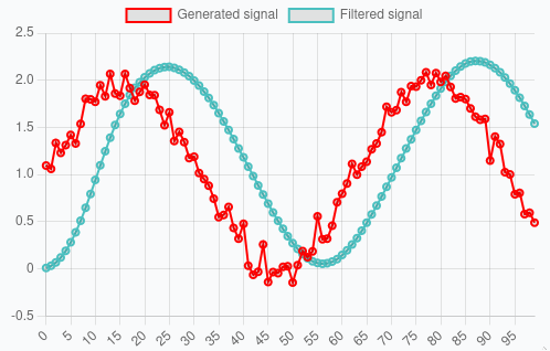
(The figure above was captured from libredsp.github.io/workspace)
For an ideal low-pass filter, the DTFT of the impulse response is as follows:
\[ H(e^{j\omega}) = \begin{cases} 1, & |\omega| < \omega_c \\ 0, & \omega_c < |\omega| \leq \pi \end{cases} \]
where \(\omega_c\) is the cutoff frequency, between \(0\) and \(\pi\). This is also called the "brick-wall" filter, because it completely passes frequencies before a certain cutoff frequency and blocks the others.
The graph of this function is depicted below:
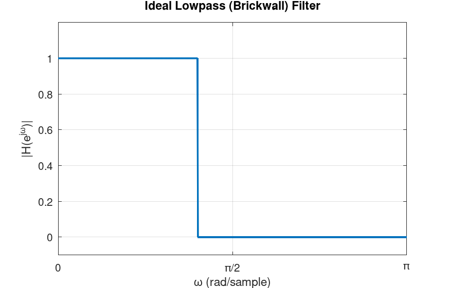
A few notes about the ideal low-pass filter. Firstly, as the figure shows, we typically plot the DTFT of the impulse response only from \(0\) to \(\pi\), because the DTFT is \(2\pi\)-periodic and, for real-valued signals and systems, we have \(H(e^{-j\omega}) = H^*(e^{j\omega})\). Moreover, the DTFT of the impulse response we saw above is in its ideal form. It can be mathematically shown that such a filter is practically not realizable. Specifically, the output of such a filter is computed by convolving the input signal \(x[n]\) in the time domain with the impulse response of this filter. The inverse DTFT of the ideal low-pass filter is "sinc-like": \[ h[n] = \frac{1}{2\pi} \int_{-\pi}^{\pi} H(e^{j\omega}) e^{j\omega n} d\omega = \frac{1}{2\pi} \int_{-\omega_c}^{\omega_c} e^{j\omega n} d\omega = \frac{\sin(\omega_c n)}{\pi n} \]
For \(n \neq 0 \) and \(h[0] = \omega_c / \pi \). This function has infinite length, therefore, to compute the convolution needed to obtain the filter's output, we need infinite computations. That being said, the filters we can design in practice can have characteristics that are very close to the ideal cases, such as the low-pass in this example.
There are numerous techniques for designing frequency-selective filters. The LibreDSP library supports the most commonly used methods including:
- The windowing method
- Zero-pole placement method
- Analog-to-digital transformation
- Least-squares linear phase FIR filters
- Parks-McClellan algorithm
Some of these methods, specifically, methods 1, 4 and 5, design finite-impulse response (FIR) filters and the rest give us infinite-impulse response (IIR) filters. Moreover, methods 1, 4 and 5 are said to have linear phase and the rest do not have this property. In the rest of this chapter we briefly talk about these differences.
FIR vs IIR Filters
A filter is said to be of type finite impulse response (FIR) if, in the LCCDE, the output \(y[n]\) depends only on the current and past input terms \(x[n], x[n-1], x[n-2], \dots\), and not on any past output terms \(y[n-k]\) for \(k \geq 1\). The word "finite" in FIR comes from the fact that if the input is the unit impulse \(\delta[n]\), the output has finite duration that is determined by the number of \(x\) terms. An example of an FIR filter is as follows:
\[ y[n] = x[n] + 0.4x[n-1] + 0.6x[n-2] \]
A filter is said to be of type infinite impulse response or IIR if the output also depends on previous output as well, meaning terms such as \(y[n-1]\), \(y[n-2]\), ..., are also present. These terms are also called feedback terms. Lastly, the word infinite in IIR stands for the infinite duration that such filters have due to delta or impulse input.
Linear Phase Filter
Having linear phase is a property that a filter can have. To understand what this property means, consider a filter when the input is \(x[n] =\cos{\omega_0 n }\). For this input, the output of the filter can be shown to be:
\[ y[n] = |H(e^{j\omega_0})| \cos\big(\omega_0 n + \angle H(e^{j\omega_0})\big) \]
where \(H(e^{j\omega})\) is the DTFT of the impulse response of the filter. What the expression above shows us is that for a pure cosine signal, the output is cosine in the same frequency but with its amplitude and phase changed by the filter. Why is the output of a filter for this particular input important? As we have discussed, for a real-valued signals (the ones we mostly deal with), their DTFT have this property:
\[ X(e^{-j\omega}) = X^*(e^{j\omega}) \]
As a consequence, in the reconstruction formula of the DTFT, for a particular frequency \(\omega_0\), we would have:
\[ A e^{j\omega_0 n} + A^* e^{-j\omega_0 n} \]
where \(A\) is some complex amplitude.
Now, writing \(A = |A| e^{j\phi}\). Then \(A^* = |A| e^{-j\phi}\). The pair becomes:
\[ |A| e^{j\phi} e^{j\omega_0 n} + |A| e^{-j\phi} e^{-j\omega_0 n} = |A| \left( e^{j(\omega_0 n + \phi)} + e^{-j(\omega_0 n + \phi)} \right) = 2|A| \cos(\omega_0 n + \phi) \]
Therefore, repeating the process above for any arbitrary frequency results in expressing any real-valued signal as a sum of real-valued cosine terms. As a consequence, knowing how the filter behaves for sinusoidal signals tells us everything we need to know about how the filter affects an arbitrary input.
Now, by definition, a filter is said to have linear phase if its frequency response has the following form:
\[ \boxed{H(e^{j\omega}) = A(\omega) e^{-j\alpha\omega}} \]
where \(A(\omega)\) is a real-valued function and \(\alpha\) is just a constant value. Substituting this expression into the expression for the output of a filter for a cosine input, for \(A(\omega_0) \ge 0\):
\[ y[n] = |A(\omega_0)| \cos\big(\omega_0 n - \omega_0 \alpha\big) = |A(\omega_0)| \cos\big(\omega_0 (n - \alpha)\big) \]
For \(A(\omega_0) \le 0\) we get an additional \(\pi\) phase shift, or equivalently: \[ y[n] = -|A(\omega_0)| \cos\big(\omega_0 (n - \alpha)\big) \]
The result of the above expressions tell us that the output of the linear phase filters due to different sinusoidal inputs, is the same sinusoid, scaled, shifted by the same amount in time or possibly with a \(\pi\) deviation.
It can be proved that filters whose impulse response is symmetric around some index or antisymmetric have linear phase. Mathematically, a symmetric filter is a filter whose impulse response is: \[ \boxed{h[n]=h[M-n] \: \: \: \: \: \text{for } 0 \leq n \leq M} \]
Where \(M\) is some index. Antisymmetric filters have the following definition:
\[ \boxed{h[n]=-h[M-n] \: \: \: \: \: \text{for } 0 \leq n \leq M} \]
Moreover, the impulse response of a symmetric and antisymmetric filter, can each be odd or even length. Therefore, depending on the symmetry and even or odd length of the impulse response we have the following four types of linear phase filters:
- Type I: Symmetric, odd length
- Type II: Symmetric, even length
- Type III: Anti-symmetric, odd length
- Type IV: Anti-symmetric, even length
Each of the four type has certain characteristics. For instance, for Type II filters, \(A(\omega)\) is always zero at \(\omega=\pi\). Consequently, they are not suited for highpass filters. In contrast, Type I filters do not have a forced zero at any frequency. Type III filters have \(A(0)=0\) and \(A(\pi)=0\). Consequently, they cannot be used for lowpass or highpass filters, but are well-suited for bandpass filters. Type IV filters, on the other hand, always have \(A(0)=0\) but no forced zero at \(\omega=\pi\). Hence, they are suitable for highpass filters.
An example of a filter with symmetric impulse response
We shall now see a simple example of a linear phase filter that has a symmetric impulse response. Assume the impulse response of the filter is symmetric with the values:
\[ h[n] = [0.1339, 0.1526, 0.1592, 0.1526, 0.1339] \]
Applying the DTFT:
\[ H(e^{j\omega}) = 0.1339 + 0.1526 e^{-j\omega} + 0.1592 e^{-j2\omega} + 0.1526 e^{-j3\omega} + 0.1339 e^{-j4\omega} \]
Factoring out \(e^{-j2\omega}\):
\[ H(e^{j\omega}) = e^{-j2\omega} \Big[ 0.1339 e^{j2\omega} + 0.1526 e^{j\omega} + 0.1592 + 0.1526 e^{-j\omega} + 0.1339 e^{-j2\omega} \Big] \]
Pairing symmetric terms using \(e^{j\theta} + e^{-j\theta} = 2 \cos(\theta) \):
\[ H(e^{j\omega}) = e^{-j2\omega} \Big[ 0.1592 + 2 \cdot 0.1339 \cos(2\omega) + 2 \cdot 0.1526 \cos(\omega) \Big] \]
Finally, we get:
\[ A(\omega) = 0.1592+ 2 [ 0.1339 \cos(2\omega)+0.1526 \cos(\omega)] \]
which is the real-valued function, and:
\[ H(e^{j\omega}) = A(\omega) e^{-j2\omega} \]
As a final remark in this subsection, for physically realizable filters, only FIR filters can have linear phase. Practical IIR filters do not have linear phase. Therefore, for applications where the linear phase property of the filter is desired, FIR filters should be used. It should also be noted that even though practical IIR filters are not linear phase, but with a small number of filter coefficients, we often can get a decent filter with sharp transitions between passband and stopband areas. This is in contrast to FIR filters that we often need 10, 20 or even more number of coefficients to produce a good filter. The magnitude and phase of this filter is depicted below:
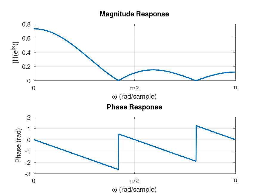
As the figure shows, the filter is a low-pass filter.
Filter Design in LibreDSP
In LibreDSP, both FIR and IIR filters with various techniques can be designed. The summary of each method is briefly mentioned below:
-
The windowing method:: Since, this is an important digital filter design technqiue both in its usage, as well as learning the filter design, the next chapter is dedicated to this method. In short, in this method, the program first obtains the impulse response of the ideal filter we would like to design, then shifts it in time by half the filter length, and multiplies the signal, element-wise, with a "window" function. The window function in the simplest form is the rectangle function. The result of multiplying the shifted impulse response with the window function is a causal impulse response. To obtain the output of the filter we then convolve an input signal with this causal impulse response. In terms of the DTFT of the output of the filter, the act of multiplying the impulse response by the window function in time, corresponds to convolution of the spectrum of the window with the ideal filter. Therefore, the larger the number of filter weights are, the larger the window would be, and the narrower its spectrum is (the uncertainty principle). As a consequence, we get a filter whose frequency response is closer to the desired frequency response. However, the larger the filter size means the larger the lag in the output of the filter.
-
Zero-pole placement method: The program receives the locations of the poles and zeroes of the Z-transform function of the desired filter, and then it gives the filter coefficients that correspond to that transfer function. This method can be helpful to visually design filters. For instance, putting poles near \(\omega=0\) and zeros around \(\omega=\pi\) will design a low pass filter.
-
Analog-to-digital transformation: For this method, the program after receiving the desired filter specification, constructs an analog filter and then discretizes it using bilinear transform. This method gives us great filters (in terms of the magnitude of the impulse response) even with a very few coefficients like with the size of 3 or 4. However, as we discussed in the last subsection, they do not have linear phase.
-
Least-squares linear phase FIR filters: The program finds the FIR filter coefficients that minimizes the square error between the designed filter and the desired filter. The program additionally can accept weighting that can weight the importance of different regions of the desired frequency segments.
-
Parks-McClellan algorithm: The program designs a 'equiripple' FIR filter using the Parks-McClellan algorithm which is essentially the Remez exchange algorithm applied to the filter design problem. The 'equiripple' property of the filter means that the errors between the designed filter and the desired filter attains a fixed maximum value related to the filter length.
The following code snippet designs a filters via LibreDSP using different methods:
use libredsp::filter_design::frequency_selective::*;
use libredsp::types::*;
use std::f64::consts::PI;
use libredsp::window::*;
fn main() {
    /* Windowing method: */

    let coefs = windowing_method(6, WindowType::Rectangular, FilterType::Lowpass { w: 0.5 });
    println!("coef {:?}", coefs);

    /* Analog-to-digital transform: */

    let coefs_iir: TransferFunction = analog_to_digital_transform_iir_filter_design(
        AnalogToDigitalTransformationDesignMethod::Butterworth,
        FilterType::Highpass { w: 0.5 },
        3,
        0.2,
    );
    println!("coef {:?}", coefs_iir);

    let fir_ls_lp = least_squares_linear_phase_fir(
        vec![0.0, 0.15, 0.85, 1.0],
        vec![1.0, 1.0, 0.0, 0.0],
        vec![1.0, 100.0],
        11,
    );
    println!("coef {:?}", fir_ls_lp);

    /* Zero-pole placement method: */
    let iir_pole_placement = zero_pole_placement_iir_filter_design(
        &vec![(0.47, -0.495), (0.47, 0.495)],
        &vec![(-0.469, -0.605), (-0.469, 0.605)],
    );
    println!("coef {:?}", iir_pole_placement);

    /* Parks-McClellan: */
    let num_taps = 11;
    let target = |f: f64| {
        if f <= 0.18 * PI { 1.0 } else { 0.0 }
    };

    let weight = |f: f64| {
        if f <= 0.18 * PI { 1.0 } else { 10.0 }
    };

    let coefficients =
        parks_mcclellan_filter_design(num_taps, target, weight, LinearPhaseFilterType::I);
    println!("{:?}", coefficients);
}
The output of the program is as follows:
coef TransferFunction { num: [0.12082847447089783, 0.14464823741432514, 0.15750225222345277, 0.15750225222345277, 0.14464823741432514, 0.12082847447089783], den: [1.0] }
coef TransferFunction { num: [0.6032341794887927, -1.8097025384663779, 1.8097025384663779, -0.6032341794887927], den: [1.0, -2.008975131286557, 1.4531076859873064, -0.363790618636477] }
coef TransferFunction { num: [0.01096242712052965, 0.015243639397498555, 0.01919520737126291, 0.02239463734598537, 0.024471842004575785, 0.025195158597253242, 0.024471842004575785, 0.02239463734598537, 0.01919520737126291, 0.015243639397498555, 0.01096242712052965], den: [1.0] }
coef TransferFunction { num: [1.0, 0.938, 0.5859859999999999], den: [1.0, -0.94, 0.465925] }
TransferFunction { num: [0.16995125386133128, 0.18332484242715108, 0.09773115654870167, 0.20681141920227245, 0.18226295845770424, 0.20848282286228859, 0.18226295845770424, 0.20681141920227245, 0.09773115654870167, 0.18332484242715108, 0.16995125386133128], den: [1.0] }
The above example shows the filter coefficients of various filters.
LibreDSP Workspace also provides a graphical user interface to design and visualize filters.
Chapter 8 - Digital Fitler Design: The Windowing Method
The last chapter introduced a several digital filter design techniques. In this chapter, we will look at the windowing method in detail. The windowing method is the simplest filter design techniques and can provides a basis to understand other filter design techniques. The windowing method allows us to design FIR filters with linear phase.
Before understanding how the windowing method works, let us first compute the impulse response of an ideal filter, and see if we can directly convolve this impulse response with an arbitrary input \(x[n]\) (remember, from the convolution theorem, doing so would perform frequency-selective filtering).
Let us assume we would like to perform lowpass filter. The impulse response of such filter has the following DTFT:
\[ H(e^{j\omega}) = \begin{cases} 1, & |\omega| < \omega_c \\ 0, & \omega_c < |\omega| \leq \pi \end{cases} \]
where \(\omega_c\) is the cutoff frequency, between \(0\) and \(\pi\).
The inverse DTFT of this expression yields:
\[ h[n] = \frac{1}{2\pi} \int_{-\pi}^{\pi} H(e^{j\omega}) e^{j\omega n} d\omega = \frac{1}{2\pi} \int_{-\omega_c}^{\omega_c} e^{j\omega n} d\omega = \frac{\sin(\omega_c n)}{\pi n} \]
For \(n \neq 0 \) and \(h[0] = \omega_c / \pi \). As a reminder from Chapter 2, the graph of this function is depicted below:
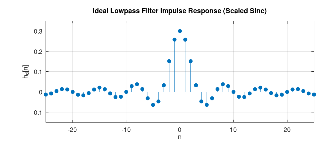
As we can see from the graph, the impulse response of such ideal filters has infinite length and is non-causal. Having infinite length means that we would require infinite computation to calculate the output of such filters via convolution. Furthermore, the non-causal nature of the impulse response means that if the input signal \(x[n]\) is being generated in real time, then its convolution with the impulse response \(h[n]\) requires access to future samples of the signal, which is physically not realizable. To understand this visually: the convolution of \(x[n]\) with the impulse response \(h[n]\) means that we fix the graph of \(x[n]\), flip \(h[n]\) with respect to the y-axis to get \(h[-n]\), shift this flipped signal, and perform element-wise multiplication and addition of the result. Now, imagine \(x[n]\) is a signal generated in real time, sample by sample, and we try to compute the convolution "on the fly" as each new sample arrives. If \(h[n]\) has non-zero values for any \(n < 0\), then when it is flipped around the y-axis, the convolution involves element-wise multiplication of some non-zero elements of \(h[n]\) with elements of \(x[n]\) that are not yet available. Therefore, the impulse response of the ideal filter we derived is not realizable. Both because of computational constraints and because it is physically unrealizable.
Note that the non-causal nature of the impulse response can be made realizable if all samples of the signal are available in advance and we perform the convolution offline. However, the infinite length of the filter still makes it computationally intractable.
The windowing method is a filter design technique that works as follows: after we derive the impulse response of an ideal filter, we shift it by an integer number of samples, we then apply "windowing", that is, we multiply the impulse response, element-wise, with a window function.
A window function, in its basic form, is simply a rectangular function defined as: \[ w[n] = \begin{cases} 1, & 0 \leq n \leq M \\ 0, & \text{otherwise} \end{cases} \] When this function is used as the window function, its effect is simply truncating the shifted impulse response.
To determine the spectrum of the impulse response of the filter designed via the windowing method, we should investigate what happens in the frequency domain when we multiply the shifted impulse response, element-wise, by the window function in the time domain. The answer lies in the use of the convolution theorem. The theorem tells us that just as multiplication in the frequency domain corresponds to convolution in the time domain, the converse is also true: multiplication in the time domain, as is the case here, corresponds to (periodic) convolution in the frequency domain.
A small note before deriving the frequency characteristic of the filters designed via the windowing method: In the process of designing filters via the windowing method, we can use different window types, such as Hann, Hamming, Bartlett, and others. Each of these window types has its own distinct effect on the resultant filter. However, a property that is common among all of them is that they are symmetric around some index. Consequently, as we saw in Chapter 4, the resulant filter will have linear phase.
A Concrete Example
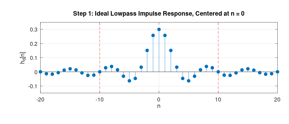
In this subsection we'll see concrete steps to design an FIR filter with the windowing method with a filter size of \(21\) and with a cutoff frequency of \(\omega_c = 0.3\) radians/samples. For simplicity, we will use the rectangular window for the design. Once we design the filter, we would also like to observe the spectrum of the filter's impulse response.
- Step 1: We would like to design a low-pass filter using the windowing method with a filter size of \(21\). To this end, we analytically find the expression for the ideal low-pass filter. As we derived at the beginning of this chapter, its impulse response is the sinc-like function. The following graph shows this infinite-length sequence (the red dots denote the desired filter size):
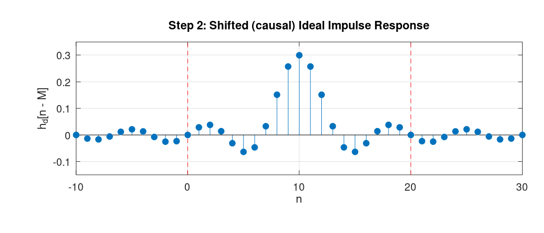
- Step 2: We shift the ideal impulse response by half the size of the desired filter (10 samples, since the filter length is 21).
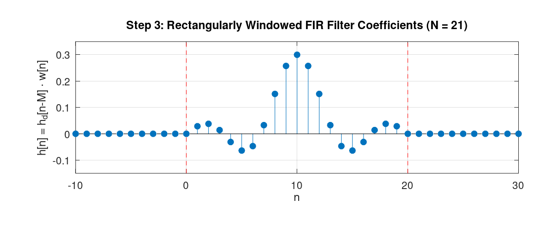
- Step 3: We apply the rectangular window with length 21 to the sequence, starting from index \(0\) to index \(20\). This gives us the filter coefficients of the desired filter.
The following graph depicts the frequency response of the designed filter.
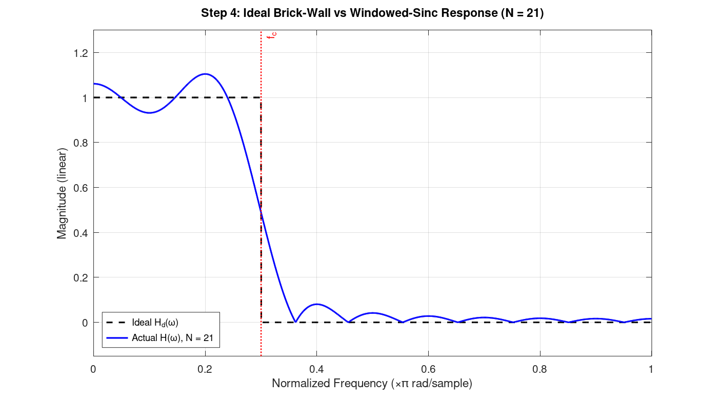
(The script that generated this graph, appended zeros to the sequence, which is referred to as "zero-padding", and then applied the DFT to the resulting sequence. From the definition of the DTFT, zero-padding and computing the DFT gives us samples of the DTFT. As we append more zeros, the result gets closer to the actual DTFT plot. Also, for computing the DFT, we typically use an efficient algorithm, such as the Fast Fourier Transform (FFT). We will learn about the FFT in Chapter 12)
As we can see, it has values close to 1 from frequency \(0\ \text{rad/sample}\) up to the cutoff frequency \(\omega_c = 0.3\) radians/samples, then decreases and reaches approximately zero. An interesting observation that can be made about the shape of the graph is that, from the convolution theorem we mentioned earlier, we know that this spectrum is the result of convolving the spectrum of the ideal filter with the spectrum of the rectangular window. The spectrum of the ideal filter is just a rectangle function in the frequency domain. The spectrum of the rectangular window (in the time domain) is a sinc-like function in the frequency domain. Consequently, the shape we see in Figure 4 is exactly the result of convolving the rectangle function with the sinc-like function.
A Few Remarks
In the example above, we chose a filter length of 21. The larger we choose this number, the closer the spectrum will be to the desired one. Specifically, the longer the rectangular function is, the more concentrated its spectrum (the sinc-like function) is around the origin. As a result, its spectrum gets convolved with a sinc-like function that has more "energy" around its point of symmetry. The resulting function has less deviation from the ideal low-pass filter in the passband and stopband regions (except at the discontinuities, in this example at \(\omega_c = 0.3\) radians/samples, because of what's known as the "Gibbs phenomenon").
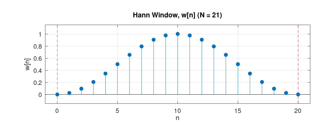
Furthermore, in the example we used the rectangular window. For comparison, we could have used another window such as the Hann window. The Hann window has the following definition: \[ w[n] = 0.5 - 0.5 \cos \left(\frac{2\pi n}{N-1}\right), \quad 0 \leq n \leq N-1 \] Below is the graph of that function for \(N = 21\):
For the design of the filter in the example, If we had used the Hann window, we would have obtained the following spectrum:
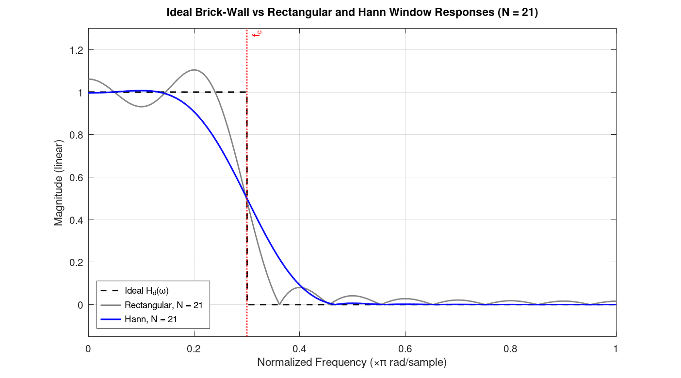
The figure shows the spectrum of the filter design by applying Han window, alongside the one obtained by applying the rectangular window as well as the ideal spectrum.
Among the window functions that are used in practice, a window called the Kaiser window has particular importance. Mathematically, it is defined as: \[ w[n] = \begin{cases} \dfrac{ I_0\!\left( \beta\sqrt{ 1-\left(\dfrac{2n}{N-1}-1\right)^2 }\right)}{I_0(\beta)}, & 0 \le n \le N-1, \\[1.2em] 0, & \text{otherwise}.\end{cases} \]
In this equation, \(I_0\) is the zeroth-order modified Bessel function of the first kind, and \(\beta\) is a parameter that is determined by the desired minimum stopband attenuation (in dB) and the transition width between the passband and stopband. Therefore, as a user, we simply provide the minimum stopband attenuation and transition width, and \(\beta\) is computed by the software automatically.
Characteristics of Filters Designed via the Windowing Method
In this section, we look at the actual formulas that tells us the spectrum of the impulse response of the filter designed via the windowing method. This section derives these expressions by applying the convolution theorem for the windowing method.
Assume the desired impulse response is symmetric and has length \(M+1\). Since it is symmetric about \(M/2\), its DTFT will be:
\[ D(e^{j\omega}) = A(e^{j\omega})\ e^{-j\omega M/2} \]
where \(A(e^{j\omega})\) is a real and even function (due to the symmetry), and \(e^{-j\omega M/2}\) denotes a delay of \(M/2\) samples in time.
Assume the window function is rectangular. Since it is also symmetric, the DTFT of this function is:
\[ W(e^{j\omega}) = B(e^{j\omega})\ e^{-j\omega M/2} \]
where \(B(e^{j\omega})\) is also real and even.
Since the window function multiplies the impulse response in time, in the frequency domain this becomes a periodic convolution:
\[ H(e^{j\omega}) = \frac{1}{2\pi} \int_{-\pi}^{\pi} W(e^{j\theta}) D(e^{j(\omega-\theta)}) d\theta \]
Substituting the two expressions into the definition of periodic convolution gives:
\[ H(e^{j\omega}) = e^{-j\omega M/2} \cdot \frac{1}{2\pi} \int_{-\pi}^{\pi} B(e^{j\theta}) A(e^{j(\omega-\theta)}) d\theta \]
(because in the convolution, the expression \(e^{-j\theta M/2} e^{-j(\omega-\theta) M/2} = e^{-j\omega M/2}\)).
The integral is a periodic convolution of two real and even functions, so the result is also real and even. Hence:
\[ H(e^{j\omega}) = C(e^{j\omega}) e^{-j\omega M/2} \]
where \(C(e^{j\omega})\) is real and even, and \(e^{-j\omega M/2}\) denotes a delay of \(M/2\) samples in time.
Chapter 9 - Statistical Filters
This chapter provides a short introduction to statistical filters. The design of statistical filters is based on the theory of random signals. A random discrete-time signal is a signal whose value at each index, \(x[n]\), is a random variable. From probability theory, we know that a random variable takes values according to some distribution, such as the exponential or Gaussian distribution. In statistical filter design, what we are concerned with is the correlation between the different values of the random signal.
As a brief introduction or recap, in general, a positive correlation between two values means that when one increases, the other tends to increase as well. Similarly, when one decreases, the other tends to decrease too. Negative correlation means the opposite: when one increases, the other tends to decrease, and vice versa. In statistical filter design, we first identify the correlation between the values of a signal in terms of auto-correlation and cross-correlation. To see how auto-correlation and cross-correlation arise in the design of statistical filters, consider the main objective in the design of such filters:
Consider a random signal as input, denoted by \(x[n]\). There is also another random signal called the desired signal, denoted by \(d[n]\). The objective of statistical filter design is to obtain the coefficients of an LCCDE such that when \(x[n]\) is used as the input of the LCCDE, the output of the filter becomes close to the desired signal \(d[n]\). This is done primarily by minimizing the expected value of the squared error, where the error is the difference between the desired signal and the output of the filter. Mathematically, if we define the error signal, \(e[n]\), as:
\[ e[n] = d[n] - y[n] \]
The objective of statistical filter design is then to minimize:
\[ E[e^2[n]] \]
Here, \(E[\cdot]\) is the expectation operator, and obtaining the above expression requires knowledge of the joint distribution, that is, the probability distribution that describes how the values of the signals behave with respect to each other. In practice, however, we use the finite data we collect to estimate this expression. For now, though, assume we know the underlying statistics of the signals and their distributions.
Also note that the desired signal \(d[n]\), depending on the problem, can be assumed to be any random signal. As a concrete example, assume that we have a system, such as an acoustic medium through which sound can propagate. With some modeling assumptions1, we would like to find the "system coefficients" that describe the dynamics of the system. 1: An assumption commonly made for such systems is that they are Linear and Time-Invariant (LTI). This means that the principle of superposition holds for such systems, meaning that a linear combination of different inputs produces the same linear combination in the output.
For such a system, the input is a random signal that we pass through the system, and the output is the signal we collect from it. For statistical filter design, we would then like to design a filter such that, when the input signal is given to the statistical filter, it produces the same output as we obtained from the system. Therefore, the input signal \(x[n]\) is the signal we gave to the unknown system, and the desired signal \(d[n]\) here refers to the output we collected from the system. The filter should produce a signal \(y[n]\) for the input \(x[n]\) that would be as close as possible to the desired signal \(d[n]\).
For the majority of statistical filter design problems, we restrict ourselves to designing FIR filters. In this case, the output of the filter is computed as:
\[ y[n] = \sum_{i=0}^{L-1} w_i x[n-i] \]
where \(w_i\) are the weights we are trying to compute. In vector form, \(W=[w_0,w_1,\ldots,w_{L-1}]^T\) and \(X[n]=[x[n],x[n-1],\ldots,x[n-L+1]]^T\), so that \(y[n]=W^TX[n]\). With this assumption, the task of minimizing the expected value of the squared error becomes:
\[ \begin{aligned} E[e^2[n]] &= E[(d[n]-W^TX[n])^2] \\ &= E[d^2[n]]-2W^Tp+W^TRW \end{aligned} \]
where \(R=E[X[n]X^T[n]]\) and \(p=E[X[n]d[n]]\).
Expanding \(R\), each entry of the matrix is:
\[ R_{ij}=E[x[n-i]x[n-j]], \quad i,j=0,1,\ldots,L-1 \]
This is called the auto-correlation matrix, and its entries represent the correlation between different values of the same random signal.
Similarly, expanding \(p\):
\[ p_i=E[x[n-i]d[n]], \quad i=0,1,\ldots,L-1 \]
This is called the cross-correlation vector. Its entries represent the correlation between values of two different signals.
Next, to find the set of coefficients \(W\) that minimizes the expected value of the squared error, we differentiate it with respect to the weights. Doing so yields:
\[ \frac{\partial E[e^2[n]]}{\partial W} =-2p+2RW=0 \]
Hence, the optimal weights are computed as:
\[ W^*=R^{-1}p \]
where \(R^{-1}\) is the inverse of the auto-correlation matrix \(R\), and \(p\) is the cross-correlation vector, provided \(R\) is invertible. Such optimal solution is called the Wiener solution.
Some note about \(R\) and \(p\)
As we have seen, the entries of the matrices \(R\) and \(p\) contain expected values \(E[...]\). Computing these terms, as we said in the previous subsection, requires knowledge of the statistical distributions of the random signals. In practice, we often do not know them and merely have a finite amount of data from such signals. To estimate these expressions using the data we collect, we then impose two assumptions in the statistical filter design problem:
(i) The signals are jointly wide-sense stationary (WSS), meaning that their means are constant and their auto-correlation and cross-correlation depend only on the "lag", i.e., the difference between the two indices.
(ii) The process is ergodic, meaning that we can estimate the "true" expected value from a single realization of the collected data.
With these assumptions, the auto-correlation of a random signal, with lag \(r=n_2-n_1\), is estimated from \(N\) samples as:
\[ R_{xx}[r]=E[x[n]x[n-r]] \approx\frac{1}{N}\sum_{n=r}^{N-1}x[n]x[n-r] \]
Similarly, the cross-correlation measures the correlation between two different signals, \(d[n]\) and \(x[n]\). Again, with the WSS and ergodicity assumptions, we can estimate it as:
\[ R_{dx}[r]=E[d[n]x[n-r]] \approx\frac{1}{N}\sum_{n=r}^{N-1}d[n]x[n-r] \]
Here, samples outside \(0,\ldots,N-1\) are unavailable, and the \(1/N\) factor makes these the biased estimators.
Wiener solution versus other statistical fitlers
The Wiener solution relies on inverting the matrix \(R\), which can be large in practice. However, inverting that matrix and multiplying it by the vector \(p\) yields the optimal solution in "one shot". If the statistics of the random signals are constantly changing, we should compute the Wiener solution iteratively on chunks of data, for instance, in fixed time intervals.
There are different algorithms to design statistical filters besides computing the Wiener solution. A famous one is called the Least Mean Squares algorithm, or LMS for short. In this method, we iteratively estimate the expected value of the squared error we defined earlier:
\[ E[e^2[n]] \]
By single data points, that is:
\[ E[e^2[n]] \approx e^2[n] = (d[n]-W^TX[n])^2 \]
This algorithm is a form of what is called an adaptive filter, because the solution is updated with every new sample, so the weights adapt over time and can track changes in the statistics of the signals. If the statistics of the random signals stay constant, the LMS solution eventually converges to the Wiener solution.
There are a variety of statistical and adaptive algorithms, such as Newton-LMS and RLS. Each algorithm has its own strengths and weaknesses, and there are tradeoffs that should be considered before choosing one.
Obtaining statistical filters in LibreDSP
The following code demonstrates using the LibreDSP library to obtain Wiener filter that recovers the coefficients of an unknown filter.
use libredsp::filter_design::statistical::{LMS, wiener};
use libredsp::signal::Signal;

fn main() {
    let mut res = Vec::with_capacity(64);

    for _ in 0..64 {
        let u1: f64 = rand::random_range(0.0..1.0);
        let u2: f64 = rand::random_range(0.0..1.0);
        let z = (-2.0 * u1.ln()).sqrt() * (2.0 * std::f64::consts::PI * u2).cos();

        res.push(z);
    }

    let x = Signal::new(res);

    // d[n] = x[n] + 0.5x[n-1], with x[-1] = 0
    let mut d = vec![0.0; x.len()];

    for n in 0..x.len() {
        d[n] = x[n] + if n > 0 { 0.5 * x[n - 1] } else { 0.0 };
    }

    let d = Signal::new(d);

    let w = wiener(&x, &d, 2);

    assert!((w[0] - 1.0).abs() < 0.05, "w[0] = {}", w[0]);
    assert!((w[1] - 0.5).abs() < 0.05, "w[1] = {}", w[1]);
}
The code above passes the asserts successfully. The above code retrives the output without any added noise, hence, it can be shown that Wiener solution gives the coefficients of the unknown filter exactly.
Chapter 10: Direction of Arrival (DOA) Estimation
When using an array of sensors, the delay between the signals received by different sensors can be used to estimate the direction of arrival (DOA) of the signal emitted by an object. For the case of two microphones, the problem of DOA estimation is depicted in the figure below. As the figure shows, the distance \(x\cos\theta\) is the additional distance that the second propagation path has to travel before reaching its microphone, compared to the first propagation path. Therefore, by estimating this time difference, we can use the following simple relation to estimate the DOA angle:
\[ \boxed{\theta=\cos^{-1}\left(\frac{c\tau_0}{x}\right)} \]
This formula comes from the equation that relates velocity to displacement. Namely, from the equations of motion, we have:
\[ \delta x = v\delta t \]
Since the speed of sound is constant, we can write:
\[ \delta x = c\tau_0 \]
Combining this with the geometric relation \(\delta x=x\cos\theta\), we obtain the above formula. A simple DOA estimation method is based on estimating the time delay \(\tau_0\) by computing the cross-correlation between the signals received by different microphones. Mathematically, the continuous-time cross-correlation function is defined as:
\[ R_{xy}(\tau) = \int_{-\infty}^{\infty}x(t)y(t+\tau),dt \]
If we assume that the signal received by the first microphone is the continuous-time function \(x(t)\), then the signal received by the second microphone is a shifted version of it, namely:
\[ s_1(t)=x(t),\qquad s_2(t)=x(t-\tau_0) \]
Therefore, the cross-correlation formula we defined above reduces to:
\[ \begin{aligned} R_{s_1s_2}(\tau) &=\int_{-\infty}^{\infty}x(t)x(t+\tau-\tau_0),dt\ &=R_{xx}(\tau-\tau_0) \end{aligned} \]
Here, because we are computing the cross-correlation of a function with itself, the resulting function is called the autocorrelation of \(x(t)\). It can be shown that the autocorrelation function \(R_{xx}(\tau)\) attains its maximum value at \(\tau=0\). Therefore, \(R_{s_1s_2}(\tau)\) attains its maximum at \(\tau=\tau_0\). Consequently, by computing the cross-correlation function and finding the argument that maximizes it, we can estimate the time delay, which in turn allows us to estimate the DOA. A problem here, however, is that when implementing the cross-correlation method on a microcontroller (MCU), the microcontroller samples continuous-time signals at regular intervals, typically integer multiples of the sampling interval \(T_s\). Because of this, we only have access to discrete values of the signals \(s_1(t)\) and \(s_2(t)\), which we denote by \(s_1[n]\) and \(s_2[n]\), respectively. Having discrete-time signals instead of continuous-time signals, the microcontroller computes the discrete-time cross-correlation function as:
\[ \boxed{ r_{s_1s_2}[\ell] =\sum_{n=-\infty}^{\infty}s_1[n]s_2[n-\ell] } \]
This expression is called the discrete-time cross-correlation. How are the values of the discrete-time cross-correlation related to those of the continuous-time cross-correlation? It can be shown that, under the condition that the signals are bandlimited and sampled at or above the Nyquist rate, the discrete-time cross-correlation function, multiplied by the sampling interval \(T_s\), gives samples of the continuous-time cross-correlation function at integer multiples of \(T_s\) 1. More precisely, with the definition of discrete-time cross-correlation used above, we have:
\[ \boxed{ R_{s_1s_2}(-\ell T_s) =T_s r_{s_1s_2}[\ell] } \]
Originally, however, we were looking for the value of \(\tau\) that maximizes the continuous-time cross-correlation function. To estimate this value using the discrete-time cross-correlation, we can take its peak value and the two neighboring samples, fit a polynomial through these three points using polynomial interpolation, and then find the maximum of that polynomial [2]. This allows us to obtain a more accurate estimate of the time delay than simply selecting the discrete sample with the maximum value.
Referencnes
Direction of Arrival (DOA) Estimation
When using an array of sensors, the delay between the signals received by different sensors in an array of sensors placed together, can be used to estimate the direction of arrival (DOA). The DOA angle refers to the angle at which the object that emitted the signal is located at, in respect to the sensor array. For the case of two microphones, the problem of DOA estimation is depicted in the figure below.
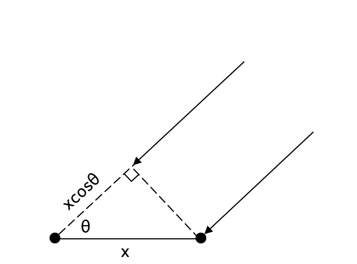
As the figure shows, the distance \(x\cos\theta\) is the additional distance that the second propagation path has to travel before reaching its microphone, compared to the first propagation path. Therefore, by estimating this time difference, we can use the following simple relation to estimate the DOA angle:
\[ \boxed{\theta=\cos^{-1}\left(\frac{c\tau_0}{x}\right)} \]
This formula comes from the equation that relates velocity to displacement. Namely, from the equations of motion, we have:
\[ \Delta x = v\Delta t \]
Since the speed of sound is constant, we can write:
\[ \Delta x = c\tau_0 \]
Combining this with the geometric relation \(\Delta x=x\cos\theta\), we obtain the above formula.
A simple DOA estimation method is based on estimating the time delay \(\tau_0\) by computing the cross-correlation between the signals received by different microphones. Mathematically, the continuous-time cross-correlation function is defined as:
\[ R_{xy}(\tau) = \int_{-\infty}^{\infty}x(t)y(t+\tau)dt \]
If we assume that the signal received by the first microphone is the continuous-time function \(x(t)\), then the signal received by the second microphone is a shifted version of it, namely:
\[ s_1(t)=x(t),\qquad s_2(t)=x(t-\tau_0) \]
Therefore, the cross-correlation formula we defined above turns into:
\[ \begin{aligned} R_{s_1s_2}(\tau) &=\int_{-\infty}^{\infty}x(t)x(t+\tau-\tau_0)dt = R_{xx}(\tau-\tau_0) \end{aligned} \]
Here, because we are computing the cross-correlation of a function with itself. The resulting function is called the auto-correlation of \(x(t)\), denoted by \(R_{xx}(\tau)\). It can be shown that the auto-correlation function \(R_{xx}(\tau)\) attains its maximum value at \(\tau=0\). Therefore, \(R_{s_1s_2}(\tau)\) attains its maximum at \(\tau=\tau_0\). Consequently, by computing the cross-correlation function and finding the argument that maximizes it, we can estimate the time delay, which in turn allows us to estimate the DOA. A problem here, however, is that when implementing the cross-correlation method on a microcontroller (MCU), the microcontroller samples continuous-time signals at regular intervals, typically integer multiples of the sampling interval \(T_s\). Because of this, we only have access to discrete values of the signals \(s_1(t)\) and \(s_2(t)\), which we denote by \(s_1[n]\) and \(s_2[n]\), respectively. Having discrete-time signals instead of continuous-time signals, the microcontroller computes the discrete-time cross-correlation function as:
\[ \boxed{ r_{s_1s_2}[\ell] =\sum_{n=-\infty}^{\infty}s_1[n]s_2[n-\ell] } \]
This expression is called the discrete-time cross-correlation.
How are the values of the discrete-time cross-correlation related to those of the continuous-time cross-correlation? It can be shown that, under the condition that the signals are bandlimited and sampled at or above the Nyquist rate, the discrete-time cross-correlation function, multiplied by the sampling interval \(T_s\), gives samples of the continuous-time cross-correlation function at integer multiples of \(T_s\) [1]. More precisely, with the definition of discrete-time cross-correlation used above, we have:
\[ \boxed{ R_{s_1s_2}(-\ell T_s) =T_s r_{s_1s_2}[\ell] } \]
In the problem of DOA estimation, however, we are looking for the value of \(\tau\) that maximizes the continuous-time cross-correlation function. To estimate this value using the discrete-time cross-correlation, we can take its peak value and the two neighboring samples, fit a polynomial through these three points using polynomial interpolation, and then find the maximum of that polynomial. This allows us to obtain a much more accurate estimate of the time delay than simply selecting the discrete sample with the maximum value.
In LibreDSP, the following example program under examples/doa_autocorrelation_based.rs performs DOA estimation on a stream of data it receives via the stdin.
This stream of data should be data of two microphones in the PCM format.
The code for this example program is as follows:
use libredsp::doa::autocorrelation_based::{DoaConfig, DoaEstimator};
use std::io::{Read, Write};

fn main() -> std::io::Result<()> {
    let config = DoaConfig::default();
    let mut estimator = DoaEstimator::new(config);

    /* One hop = hop_size frames * 2 channels * 2 bytes. */
    let mut buf = vec![0u8; config.hop_size * 4];
    let mut stdin = std::io::stdin().lock();

    eprintln!("Waiting for audio on stdin...");

    while stdin.read_exact(&mut buf).is_ok() {
        let samples: Vec<i16> = buf
            .chunks_exact(2)
            .map(|b| i16::from_le_bytes([b[0], b[1]]))
            .collect();

        for e in estimator.push_interleaved_i16(&samples) {
            match e.angle_degrees {
                Some(a) => print!("DOA: {:+7.2} degrees ({:.1} dBFS)       \r", a, e.dbfs),
                None => print!("INACTIVE ({:.1} dBFS)       \r", e.dbfs),
            }
            std::io::stdout().flush()?;
        }
    }
    Ok(())
}
This example can be used, for instance, by redirecting data that is received from the microcontroller via the USB serial connection to this program.
To do this, the host's USB serial diver has to be configured to match the microcontroller data transmission baud-rate.
Afterwards, the port that the data is being received on the host can be read via the cat command, and then be redirected to the example program above.
These steps can be done with similar commands to following ones:
stty -F /dev/ttyUSB0 921600 raw -echo
cat /dev/ttyUSB0 | cargo run --release --example doa_autocorrelation_based
The output of the program would then similar to:
DOA: +80.6 degrees (-31.9 dBFS)
You can then configure the USB serial input driver in your system to receive the data with the baud-rate that
Referencnes
[1] Butzer, P. L., et al. The sampling theorem, Poisson's summation formula, general Parseval formula, reproducing kernel formula and the Paley–Wiener theorem for bandlimited signals–their interconnections. Applicable Analysis 90.3-4 (2011): 431-461.