Direction of Arrival (DOA) Estimation
When using an array of sensors, the delay between the signals received by different sensors in an array of sensors placed together, can be used to estimate the direction of arrival (DOA). The DOA angle refers to the angle at which the object that emitted the signal is located at, in respect to the sensor array. For the case of two microphones, the problem of DOA estimation is depicted in the figure below.
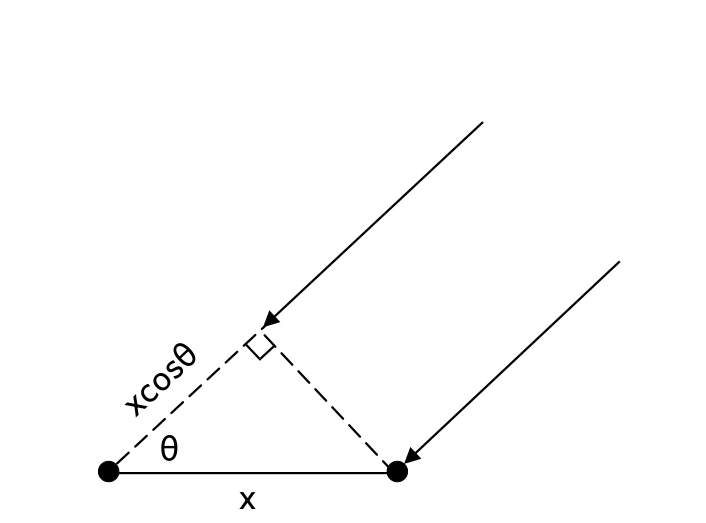
As the figure shows, the distance \(x\cos\theta\) is the additional distance that the second propagation path has to travel before reaching its microphone, compared to the first propagation path. Therefore, by estimating this time difference, we can use the following simple relation to estimate the DOA angle:
\[ \boxed{\theta=\cos^{-1}\left(\frac{c\tau_0}{x}\right)} \]
This formula comes from the equation that relates velocity to displacement. Namely, from the equations of motion, we have:
\[ \Delta x = v\Delta t \]
Since the speed of sound is constant, we can write:
\[ \Delta x = c\tau_0 \]
Combining this with the geometric relation \(\Delta x=x\cos\theta\), we obtain the above formula.
A simple DOA estimation method is based on estimating the time delay \(\tau_0\) by computing the cross-correlation between the signals received by different microphones. Mathematically, the continuous-time cross-correlation function is defined as:
\[ R_{xy}(\tau) = \int_{-\infty}^{\infty}x(t)y(t+\tau)dt \]
If we assume that the signal received by the first microphone is the continuous-time function \(x(t)\), then the signal received by the second microphone is a shifted version of it, namely:
\[ s_1(t)=x(t),\qquad s_2(t)=x(t-\tau_0) \]
Therefore, the cross-correlation formula we defined above turns into:
\[ \begin{aligned} R_{s_1s_2}(\tau) &=\int_{-\infty}^{\infty}x(t)x(t+\tau-\tau_0)dt = R_{xx}(\tau-\tau_0) \end{aligned} \]
Here, because we are computing the cross-correlation of a function with itself. The resulting function is called the auto-correlation of \(x(t)\), denoted by \(R_{xx}(\tau)\). It can be shown that the auto-correlation function \(R_{xx}(\tau)\) attains its maximum value at \(\tau=0\). Therefore, \(R_{s_1s_2}(\tau)\) attains its maximum at \(\tau=\tau_0\). Consequently, by computing the cross-correlation function and finding the argument that maximizes it, we can estimate the time delay, which in turn allows us to estimate the DOA. A problem here, however, is that when implementing the cross-correlation method on a microcontroller (MCU), the microcontroller samples continuous-time signals at regular intervals, typically integer multiples of the sampling interval \(T_s\). Because of this, we only have access to discrete values of the signals \(s_1(t)\) and \(s_2(t)\), which we denote by \(s_1[n]\) and \(s_2[n]\), respectively. Having discrete-time signals instead of continuous-time signals, the microcontroller computes the discrete-time cross-correlation function as:
\[ \boxed{ r_{s_1s_2}[\ell] =\sum_{n=-\infty}^{\infty}s_1[n]s_2[n-\ell] } \]
This expression is called the discrete-time cross-correlation.
How are the values of the discrete-time cross-correlation related to those of the continuous-time cross-correlation? It can be shown that, under the condition that the signals are bandlimited and sampled at or above the Nyquist rate, the discrete-time cross-correlation function, multiplied by the sampling interval \(T_s\), gives samples of the continuous-time cross-correlation function at integer multiples of \(T_s\) [1]. More precisely, with the definition of discrete-time cross-correlation used above, we have:
\[ \boxed{ R_{s_1s_2}(-\ell T_s) =T_s r_{s_1s_2}[\ell] } \]
In the problem of DOA estimation, however, we are looking for the value of \(\tau\) that maximizes the continuous-time cross-correlation function. To estimate this value using the discrete-time cross-correlation, we can take its peak value and the two neighboring samples, fit a polynomial through these three points using polynomial interpolation, and then find the maximum of that polynomial. This allows us to obtain a much more accurate estimate of the time delay than simply selecting the discrete sample with the maximum value.
In LibreDSP, the following example program under examples/doa_autocorrelation_based.rs performs DOA estimation on a stream of data it receives via the stdin.
This stream of data should be data of two microphones in the PCM format.
The code for this example program is as follows:
use libredsp::doa::autocorrelation_based::{DoaConfig, DoaEstimator};
use std::io::{Read, Write};

fn main() -> std::io::Result<()> {
    let config = DoaConfig::default();
    let mut estimator = DoaEstimator::new(config);

    /* One hop = hop_size frames * 2 channels * 2 bytes. */
    let mut buf = vec![0u8; config.hop_size * 4];
    let mut stdin = std::io::stdin().lock();

    eprintln!("Waiting for audio on stdin...");

    while stdin.read_exact(&mut buf).is_ok() {
        let samples: Vec<i16> = buf
            .chunks_exact(2)
            .map(|b| i16::from_le_bytes([b[0], b[1]]))
            .collect();

        for e in estimator.push_interleaved_i16(&samples) {
            match e.angle_degrees {
                Some(a) => print!("DOA: {:+7.2} degrees ({:.1} dBFS)       \r", a, e.dbfs),
                None => print!("INACTIVE ({:.1} dBFS)       \r", e.dbfs),
            }
            std::io::stdout().flush()?;
        }
    }
    Ok(())
}
This example can be used, for instance, by redirecting data that is received from the microcontroller via the USB serial connection to this program.
To do this, the host's USB serial diver has to be configured to match the microcontroller data transmission baud-rate.
Afterwards, the port that the data is being received on the host can be read via the cat command, and then be redirected to the example program above.
These steps can be done with similar commands to following ones:
stty -F /dev/ttyUSB0 921600 raw -echo
cat /dev/ttyUSB0 | cargo run --release --example doa_autocorrelation_based
The output of the program would then similar to:
DOA: +80.6 degrees (-31.9 dBFS)
You can then configure the USB serial input driver in your system to receive the data with the baud-rate that
Referencnes
[1] Butzer, P. L., et al. The sampling theorem, Poisson's summation formula, general Parseval formula, reproducing kernel formula and the Paley–Wiener theorem for bandlimited signals–their interconnections. Applicable Analysis 90.3-4 (2011): 431-461.